Tutorial
Welcome to this tutorial on using OpenFLASH! This guide demonstrates how to set up a multi-body hydrodynamic problem, run the simulation engine, and analyze the results.
OpenFLASH uses the Matched Eigenfunction Expansion Method (MEEM) to efficiently analyze wave interactions with concentric structures, providing key hydrodynamic insights like added mass, damping, and potential fields.
1. Prerequisites and Setup
Before you begin, make sure you have installed the openflash package. If you haven’t, you can install it using pip. It’s highly recommended to do this within a virtual environment.
# Install the package from your local project directory
pip install open-flash
[1]:
import numpy as np
import matplotlib.pyplot as plt
import pandas as pd
import openflash
print(type(openflash))
print(openflash.__path__)
print(openflash.__file__)


# --- Import core modules from package ---
try:
    from openflash import *
    from openflash.multi_constants import g
    print("OpenFLASH modules imported successfully!")
except ImportError as e:
    print(f"Error importing OpenFLASH modules. Error: {e}")

# Set NumPy print options for better readability
np.set_printoptions(threshold=np.inf, linewidth=np.inf, precision=8, suppress=True)
<class 'module'>
['/Users/hopebest/Documents/semi-analytical-hydro/package/src/openflash']
/Users/hopebest/Documents/semi-analytical-hydro/package/src/openflash/__init__.py
OpenFLASH modules imported successfully!
[2]:
# ---------------------------------
# --- 1. Problem Setup ---
# ---------------------------------
print("\n--- 1. Setting up the Problem ---")
h = 1.001            # Water Depth (m)
d_list = [0.5, 0.25]   # Step depths (m) for inner and outer bodies
a_list = [0.5, 1.0]    # Radii (m) for inner and outer bodies
NMK = [30, 30, 30]     # Harmonics for inner, middle, and exterior domains

m0 = 1.0    # Non-dimensional wave number
problem_omega = omega(m0, h, g)
print(f"Wave number (m0): {m0}, Angular frequency (omega): {problem_omega:.4f}")
--- 1. Setting up the Problem ---
Wave number (m0): 1.0, Angular frequency (omega): 2.7341
[3]:
def run_simulation(heaving_list, case_name):
    """Sets up geometry, problem, and engine for a specific heaving configuration."""
    print(f"\n--- Running Simulation: {case_name} ---")

    # 1. Create Bodies
    bodies = []
    for i in range(len(a_list)):
        body = SteppedBody(
            a=np.array([a_list[i]]),
            d=np.array([d_list[i]]),
            slant_angle=np.array([0.0]),
            heaving=heaving_list[i]
        )
        bodies.append(body)

    # 2. Arrangement
    arrangement = ConcentricBodyGroup(bodies)

    # 3. Geometry
    geometry = BasicRegionGeometry(
        body_arrangement=arrangement,
        h=h,
        NMK=NMK
    )

    # 4. Problem
    problem = MEEMProblem(geometry)
    problem.set_frequencies(np.array([problem_omega]))

    # 5. Engine
    engine = MEEMEngine(problem_list=[problem])

    # 6. Solve
    print(f"Solving for {case_name}...")
    X = engine.solve_linear_system_multi(problem, m0)

    # 7. Coefficients
    coeffs = engine.compute_hydrodynamic_coefficients(problem, X, m0)

    return problem, X, coeffs
2. Case 1: Inner Body Heaving (Mode 0)
We simulate the case where only the inner body is heaving (heaving_list = [True, False]).
[4]:
problem1, X1, coeffs1 = run_simulation([True, False], "Inner Body Heaving")

print("\nHydrodynamic Coefficients (Mode 0):")
if coeffs1:
    print(pd.DataFrame(coeffs1))
--- Running Simulation: Inner Body Heaving ---
Solving for Inner Body Heaving...

Hydrodynamic Coefficients (Mode 0):
   mode        real        imag  excitation_phase  excitation_force
0     0  288.113192  188.447876         -0.521015         63.283109
1     1  593.957964  590.899836         -0.521015         84.210930
/Users/hopebest/Documents/semi-analytical-hydro/.venv/lib/python3.12/site-packages/scipy/_lib/_util.py:1233: LinAlgWarning: Ill-conditioned matrix (rcond=6.46955e-30): result may not be accurate.
  return f(*arrays, *other_args, **kwargs)
3. Case 2: Outer Body Heaving (Mode 1)
Now we simulate the case where only the outer body is heaving (heaving_list = [False, True]).
Note: Currently, the package calculates the diagonal terms of the hydrodynamic coefficient matrix. Off-diagonal (coupling) terms are not yet implemented, so we run separate problems for each mode.
[5]:
problem2, X2, coeffs2 = run_simulation([False, True], "Outer Body Heaving")

print("\nHydrodynamic Coefficients (Mode 1):")
if coeffs2:
    print(pd.DataFrame(coeffs2))
--- Running Simulation: Outer Body Heaving ---
Solving for Outer Body Heaving...

Hydrodynamic Coefficients (Mode 1):
   mode        real         imag  excitation_phase  excitation_force
0     0  341.504733   590.899825         -0.521015         84.210929
1     1  930.881906  1852.833881         -0.521015        112.059612
/Users/hopebest/Documents/semi-analytical-hydro/.venv/lib/python3.12/site-packages/scipy/_lib/_util.py:1233: LinAlgWarning: Ill-conditioned matrix (rcond=6.46955e-30): result may not be accurate.
  return f(*arrays, *other_args, **kwargs)
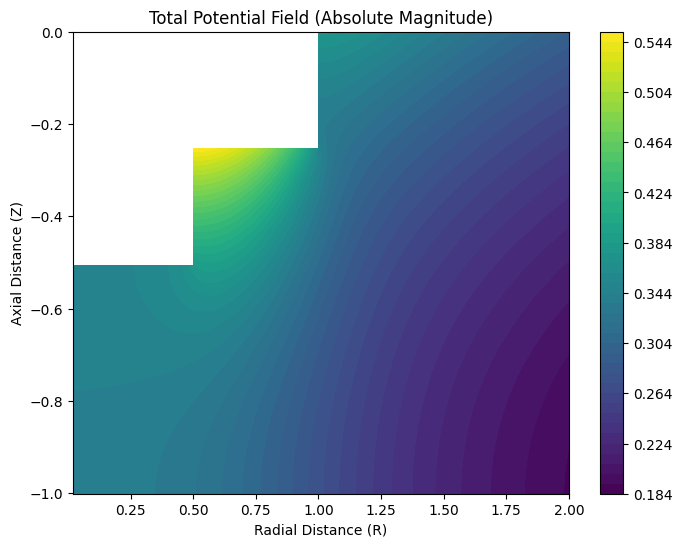
4. Potential Field Visualization
We can visualize the potential field for Case 2 (Outer Body Heaving).
[6]:
# 1. Re-initialize Engine for Visualization
engine_viz = MEEMEngine([problem2])

# 2. Calculate Potentials
print("Calculating potentials on grid...")
potentials = engine_viz.calculate_potentials(
    problem=problem2,
    solution_vector=X2,
    m0=m0,
    spatial_res=100,
    sharp=True
)

# 3. Extract Fields
R = potentials['R']
Z = potentials['Z']
phi_abs = np.abs(potentials['phi'])

# 4. Plot
print("Plotting...")
fig, ax = engine_viz.visualize_potential(phi_abs, R, Z, "Total Potential Field (Absolute Magnitude)")
plt.show()
Calculating potentials on grid...
Plotting...
5. Domain Analysis
We can inspect the fluid domains created by the BasicRegionGeometry.
[7]:
print("\n--- Inspecting Fluid Domains ---")
domains = problem2.geometry.domain_list

for idx, domain in domains.items():
    print(f"Domain {idx} ({domain.category}):")
    outer_str = f"{domain.a_outer:.2f}" if domain.a_outer != np.inf else "inf"
    print(f"  Radii: {domain.a_inner:.2f} m to {outer_str} m")
    print(f"  Lower Depth: {domain.d_lower:.2f} m")
    print(f"  Harmonics: {domain.number_harmonics}")
--- Inspecting Fluid Domains ---
Domain 0 (interior):
  Radii: 0.00 m to 0.50 m
  Lower Depth: 0.50 m
  Harmonics: 30
Domain 1 (interior):
  Radii: 0.50 m to 1.00 m
  Lower Depth: 0.25 m
  Harmonics: 30
Domain 2 (exterior):
  Radii: 1.00 m to inf m
  Lower Depth: 0.00 m
  Harmonics: 30
6. Storing and Exporting Results
The Results class (based on xarray) provides a structured way to store simulation data. Since we ran two separate simulations (one per mode), we will manually aggregate the results into a single dataset containing the full 2x2 added mass and damping matrices.
[8]:
# 1. Initialize Results object for the FULL system
# We explicitly pass the modes [0, 1] so the container can hold the full matrix,
# even though problem2 only had mode 1 active.
all_modes = np.arange(len(a_list)) # [0, 1]
results = Results(problem2, modes=all_modes)

# 2. Construct Full Matrices from Separate Mode Results
# Shape: (n_freqs, n_modes, n_modes)
n_freqs = len(problem2.frequencies)
n_modes = len(all_modes)

added_mass = np.zeros((n_freqs, n_modes, n_modes))
damping = np.zeros((n_freqs, n_modes, n_modes))

# Helper to fill matrix columns
# coeffs_list contains entries for row_idx (force on body i)
# col_idx (motion of body j) is determined by which case we ran
def fill_matrix_col(coeffs_list, col_idx):
    for c in coeffs_list:
        row_idx = c['mode'] # Force on body i
        added_mass[0, row_idx, col_idx] = c['real']
        damping[0, row_idx, col_idx] = c['imag']

# Fill Column 0 (Inner Body Heaving results -> Mode 0)
if coeffs1:
    fill_matrix_col(coeffs1, 0)

# Fill Column 1 (Outer Body Heaving results -> Mode 1)
if coeffs2:
    fill_matrix_col(coeffs2, 1)

# 3. Store in Results Object
results.store_hydrodynamic_coefficients(
    frequencies=problem2.frequencies,
    added_mass_matrix=added_mass,
    damping_matrix=damping
)

# 4. View Dataset
print("\n--- Results Dataset (xarray) ---")
print(results.dataset)

# 5. Export (Optional)
# results.export_to_netcdf("tutorial_results.nc")
Hydrodynamic coefficients stored in xarray dataset.

--- Results Dataset (xarray) ---
<xarray.Dataset> Size: 104B
Dimensions:     (frequency: 1, mode_i: 2, mode_j: 2)
Coordinates:
  * frequency   (frequency) float64 8B 2.734
  * mode_i      (mode_i) int64 16B 0 1
  * mode_j      (mode_j) int64 16B 0 1
Data variables:
    added_mass  (frequency, mode_i, mode_j) float64 32B 288.1 341.5 594.0 930.9
    damping     (frequency, mode_i, mode_j) float64 32B 188.4 ... 1.853e+03